Simulation and identification of RC circut

New small project: simulation and identification RC circuit in Python. Jupyter notebook could be found here. First part was simulation. Then I used STM32discovery to catch some real data and identify parameters.

First part of this post will by about simulating basic RC circuit. We start from differential equation and then calculate transfer function. Secound part will be comparing step response of iurs modeal and real RC-circuit. All simulation was done in Python.

First we need to load librarys:

import numpy
import scipy
import matplotlib.pyplot as plt
%matplotlib inline
from sympy import init_session
init_session() 
import scipy.signal as sig
import scipy.optimize as opt
from IPython.display import Image

IPython console for SymPy 1.0 (Python 3.5.2-64-bit) (ground types: python)

These commands were executed:
>>> from __future__ import division
>>> from sympy import *
>>> x, y, z, t = symbols('x y z t')
>>> k, m, n = symbols('k m n', integer=True)
>>> f, g, h = symbols('f g h', cls=Function)
>>> init_printing()

Documentation can be found at http://docs.sympy.org/1.0/

Equations

The scheme of circuit is shown in belowe figure:

title

The input is of system is $u(t)$ . The output $y(t)$ is voltage on capasitor. $R$ is resistance in Ohms and $C$ capacity in Farads. $q(t)$ is the charge on capacitor. From Ohms and Kirchoffs laws we could get equations:

t = symbols('t')
u = Function('u')(t)
x = Function('x')(t)
y = Function('y')(t)
R, C = symbols('R C')
equations = [Eq(u, R*Derivative(x, t)+x/C), Eq(y, x/C)]
equations

$\left [ u{\left (t \right )} = R \frac{d}{d t} x{\left (t \right )} + \frac{1}{C} x{\left (t \right )}, \quad y{\left (t \right )} = \frac{1}{C} x{\left (t \right )}\right ]$

The we gen calculate Laplace transform of our equation. Simpy currently can not do that, so we performe it manualy. $G(s)$ will be transfer function of this system.

s = symbols('s')
U = Function('U')(s)
X = Function('X')(s)
Y = Function('Y')(s)
L_equations = [Eq(U, R*X*s+X/C), Eq(Y, X/C)]
L_equations

$\left [ U{\left (s \right )} = R s X{\left (s \right )} + \frac{1}{C} X{\left (s \right )}, \quad Y{\left (s \right )} = \frac{1}{C} X{\left (s \right )}\right ]$

Then we could solve this system of equations and get transfer function:

L_s = solve(L_equations,Y,X)
G = L_s[Y]/U
G

$\frac{1}{C R s + 1}$

We get first order objet. Now we choose values for parameters and create transfer function for futures calculations:

R_v = 100000
C_v =  100e-9
G_RC = G.subs(R, R_v).subs(C, C_v)
G_RC

$\frac{1}{0.01 s + 1}$

num = Poly(fraction(G_RC)[0], s).all_coeffs()
num = [float(i) for i in num]
num = numpy.array(num)
den = Poly(fraction(G_RC)[1], s).all_coeffs()
den = [float(i) for i in den]
den = numpy.array(den)
G_n = sig.TransferFunction(num, den)

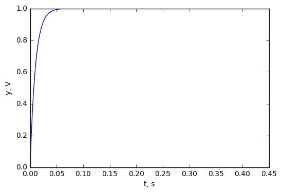
Now we could draw step response of our system:

t = numpy.linspace(0, 0.4, 401)
step_response=G_n.step(T=t)
%matplotlib inline
fig = plt.axes()
fig.plot(step_response[0], step_response[1])
fig.set_xlabel('t, s')
fig.set_ylabel('y, V')

<matplotlib.text.Text at 0x1f1a8a9f198>

png

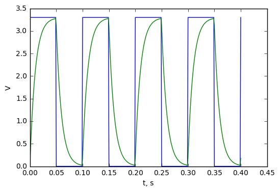
And last simulation - respons for square wave:

pwm = 3.3*(sig.square(2*numpy.pi*10*t)+1)/2
response = G_n.output(pwm, T=t)
fig = plt.axes()
fig.plot(t, pwm, t, response[1])
fig.set_xlabel('t, s')
fig.set_ylabel('V')

<matplotlib.text.Text at 0x1f1a88c6518>

png

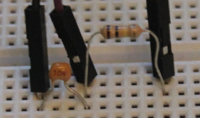
Experiment

Simple program for STM32F401 was write. It generate pwm signal and gather voltage from capacitor by 12 bit ADC with frequwncy $1~kHz$ . Belowe photo show measurements set-up:

title

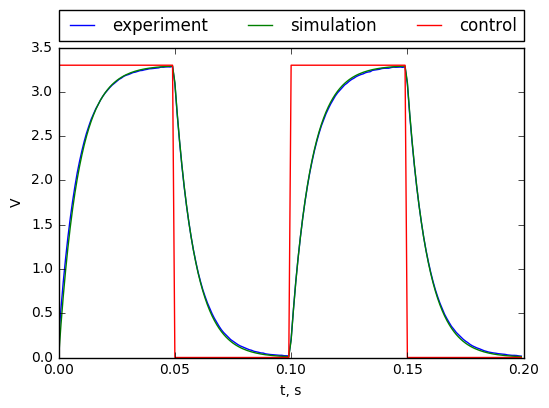
Comparision beetween experimantal and simulated data is dhown in figure belowe:

data = np.transpose(np.loadtxt('data.txt'));
data[0] = 3.3*data[0]/(2**12-1)
fig = plt.axes()
experiment, = fig.plot(t[0:200], data[0][0:200], label='experiment')
simulation, = fig.plot(t[0:200], response[1][0:200], label='simulation')
control, = fig.plot(t[0:200], pwm[0:200], label = 'control')
plt.legend(handles=[experiment, simulation, control])
plt.legend(bbox_to_anchor=(0., 1.02, 1., .102), loc=3,
           ncol=3, mode="expand", borderaxespad=0.)
fig.set_xlabel('t, s')
fig.set_ylabel('V')

<matplotlib.text.Text at 0x1f1a8ad5518>

png

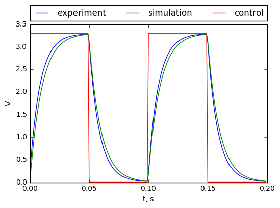
The mean squear error beetween simulation and data:

MSE = numpy.sum(numpy.power(data[0][0:200]-response[1][0:200], 2))
MSE

$2.78395309908$

We could optimize value of $RC$ for best fit to data. I measured value of $R$ and got $101.3~k\Omega$ , so this method could be used to obtain $C$ .

def ErrorFunc(RC):
    t = numpy.linspace(0, 0.2, 201)
    pwm = 3.3*(sig.square(2*numpy.pi*10*t)+1)/2
    G_n = sig.TransferFunction(np.array([1]), np.array([RC[0], 1]))
    res = G_n.output(pwm, T=t)
    return numpy.sum(numpy.power(data[0][0:200]-res[1][0:200], 2))

ErrorFunc(np.array([R_v*C_v]))

$2.78395309908$

output = opt.least_squares(ErrorFunc, np.array([R_v*C_v]))
[output.x, ErrorFunc(output.x)]

[array([ 0.00847335]), 0.21172472224806402]

Now it is possible to calculete exact value of $C$ :

output.x[0]/101300

$8.3646141698e-08$

So the capacity is aobiut $83.6~nF$ . Comparison of respons of simulation and data is shown belowe:

G_opt = sig.TransferFunction(np.array([1]), np.array([output.x[0], 1]))
res_opt = G_opt.output(pwm, T=t)
fig = plt.axes()
experiment, = fig.plot(t[0:200], data[0][0:200], label='experiment')
simulation, = fig.plot(t[0:200], res_opt[1][0:200], label='simulation')
control, = fig.plot(t[0:200], pwm[0:200], label = 'control')
plt.legend(handles=[experiment, simulation, control])
plt.legend(bbox_to_anchor=(0., 1.02, 1., .102), loc=3,
           ncol=3, mode="expand", borderaxespad=0.)
fig.set_xlabel('t, s')
fig.set_ylabel('V')

<matplotlib.text.Text at 0x1f1aa7c1470>

png

Summary

This notebook cover some interesting python features: symbolic calculations, simulation of the transfer functions and last but not list identification of simple, but real dynamic system. I measure the capacity by multimeter and get value $89.3~nF$ , so achived result is nod very good. But data from model rather good fit to data. Model was build on breadboard so there could be parasitic capacitance and resistance.

Written on November 19, 2016